Plot quantile-quantile (QQ) graphs from residuals of linear models.
Source:R/plot_qqmodel.R
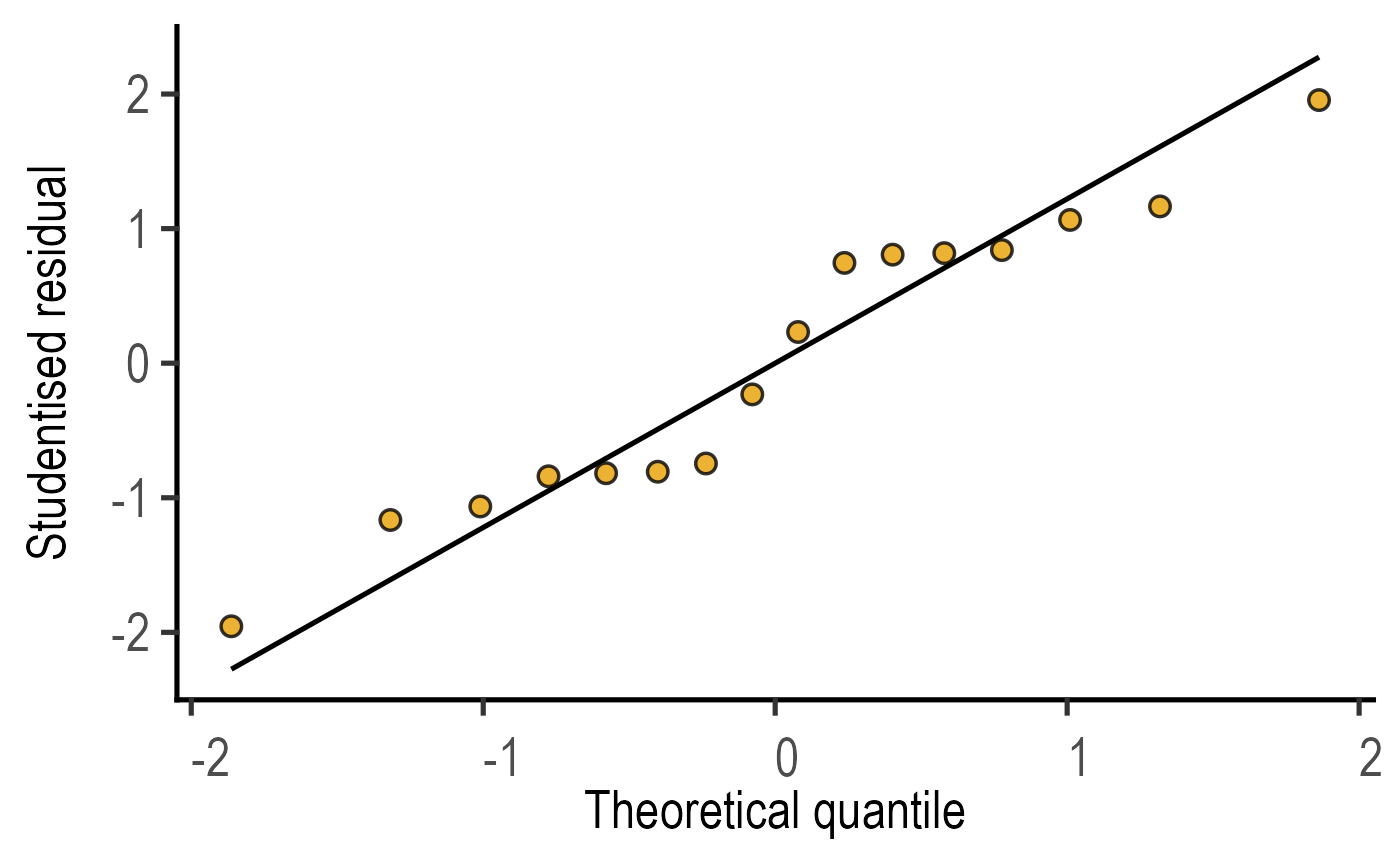
plot_qqmodel.RdThis function takes a linear model (simple or mixed effects) and plots a QQ graph after running rstudent from rstudent to generate a table of Studentised model residuals on an ordinary (simple_model), mixed model (mixed_model or mixed_model_slopes. The graph plots studentised residuals from the model (sample) on Y axis & Theoretical quantiles on X axis.
plot_qqmodel(
  Model,
  symsize = 3,
  s_alpha = 0.8,
  fontsize = 20,
  symthick,
  linethick,
  SingleColour = "#E69F00"
)
Arguments
- Model
name of a saved model generated by
simple_modelormixed_model.- symsize
size of symbols, default set to 3.
- s_alpha
fractional opacity of symbols, default set to 0.8 (i.e., 80% opacity).
- fontsize
parameter of
base_sizeof fonts intheme_classic, default set to size 20.- symthick
thickness of symbol border, default set to
fontsize/22.- linethick
thickness of line, default set to
fontsize/22.- SingleColour
colour of symbols (default =
#E69F00, which isok_orange)
Value
This function returns a ggplot2 object of class "gg" and "ggplot".
Details
For generalised additive models fit with mgcv, scaled Pearson residuals are plotted.
The function uses geom_qq and geom_qq_line geometries. Symbols receive "ok_orange" colour by default.
Examples
#Basic usage
m1 <- simple_model(data = data_2w_Festing,
Y_value = "GST",
Fixed_Factor = c("Treatment", "Strain"))
plot_qqmodel(m1)