This function takes a data table, ycol of quantitative variable and a categorical grouping variable (group), if available, and plots a density graph using geom_density). Alternatives are plot_histogram, or plot_qqline.
plot_density(
  data,
  ycol,
  group,
  facet,
  PlotType = c("Density", "Counts", "Normalised counts"),
  c_alpha = 0.2,
  TextXAngle = 0,
  facet_scales = "fixed",
  fontsize = 20,
  linethick,
  LogYTrans,
  LogYBreaks = waiver(),
  LogYLabels = waiver(),
  LogYLimits = NULL,
  ColPal = c("okabe_ito", "all_grafify", "bright", "contrast", "dark", "fishy", "kelly",
    "light", "muted", "pale", "r4", "safe", "vibrant"),
  ColSeq = TRUE,
  ColRev = FALSE,
  SingleColour = NULL,
  ...
)
Arguments
- data
a data table e.g. data.frame or tibble.
- ycol
name of the column (without quotes) with the quantitative variable whose density distribution is to be plotted.
- group
name of the column containing a categorical grouping variable (optional Since v5.0.0).
- facet
add another variable (without quotes) from the data table to create faceted graphs using
facet_wrap.- PlotType
the default (
Density) plot will be the probability density curve, which can be changed toCountsorNormalised counts.- c_alpha
fractional opacity of filled colours under the curve, default set to 0.2 (i.e. 20% opacity).
- TextXAngle
orientation of text on X-axis; default 0 degrees. Change to 45 or 90 to remove overlapping text.
- facet_scales
whether or not to fix scales on X & Y axes for all facet facet graphs. Can be
fixed(default),free,free_yorfree_x(for Y and X axis one at a time, respectively).- fontsize
parameter of
base_sizeof fonts intheme_classic, default set to size 20.- linethick
thickness of symbol border, default set to
fontsize/22.- LogYTrans
transform Y axis into "log10" or "log2" (in quotes).
- LogYBreaks
argument for
scale_y_continuousfor Y axis breaks on log scales, default iswaiver(), or provide a vector of desired breaks.- LogYLabels
argument for
scale_y_continuousfor Y axis labels on log scales, default iswaiver(), or provide a vector of desired labels.- LogYLimits
a vector of length two specifying the range (minimum and maximum) of the Y axis.
- ColPal
grafify colour palette to apply (in quotes), default "okabe_ito"; see
graf_palettesfor available palettes.- ColSeq
logical TRUE or FALSE. Default TRUE for sequential colours from chosen palette. Set to FALSE for distant colours, which will be applied using
scale_fill_grafify2.- ColRev
whether to reverse order of colour within the selected palette, default F (FALSE); can be set to T (TRUE).
- SingleColour
a colour hexcode (starting with #, e.g., "#E69F00"), a number between 1-154, or names of colours from
grafifypalettes or base R to fill along X-axis aesthetic. Accepts any colour other than "black"; usegrey_lin11, which is almost black.- ...
any additional arguments to pass to
geom_density.
Value
This function returns a ggplot2 object of class "gg" and "ggplot".
Details
Note that the function requires the quantitative Y variable first, and groups them based on an X variable. The group variable is mapped to the fill and colour aesthetics in geom_density.
Colours can be changed using ColPal, ColRev or ColSeq arguments. Colours available can be seen quickly with plot_grafify_palette.
ColPal can be one of the following: "okabe_ito", "dark", "light", "bright", "pale", "vibrant, "muted" or "contrast".
ColRev (logical TRUE/FALSE) decides whether colours are chosen from first-to-last or last-to-first from within the chosen palette.
ColSeq decides whether colours are picked by respecting the order in the palette or the most distant ones using colorRampPalette.
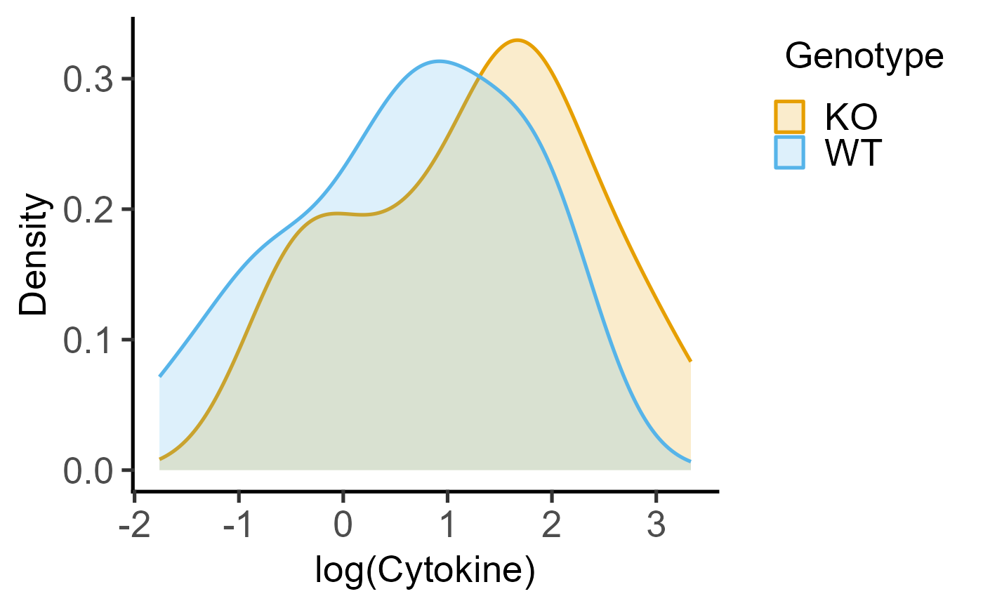
Examples
plot_density(data = data_t_pratio,
ycol = log(Cytokine), group = Genotype)
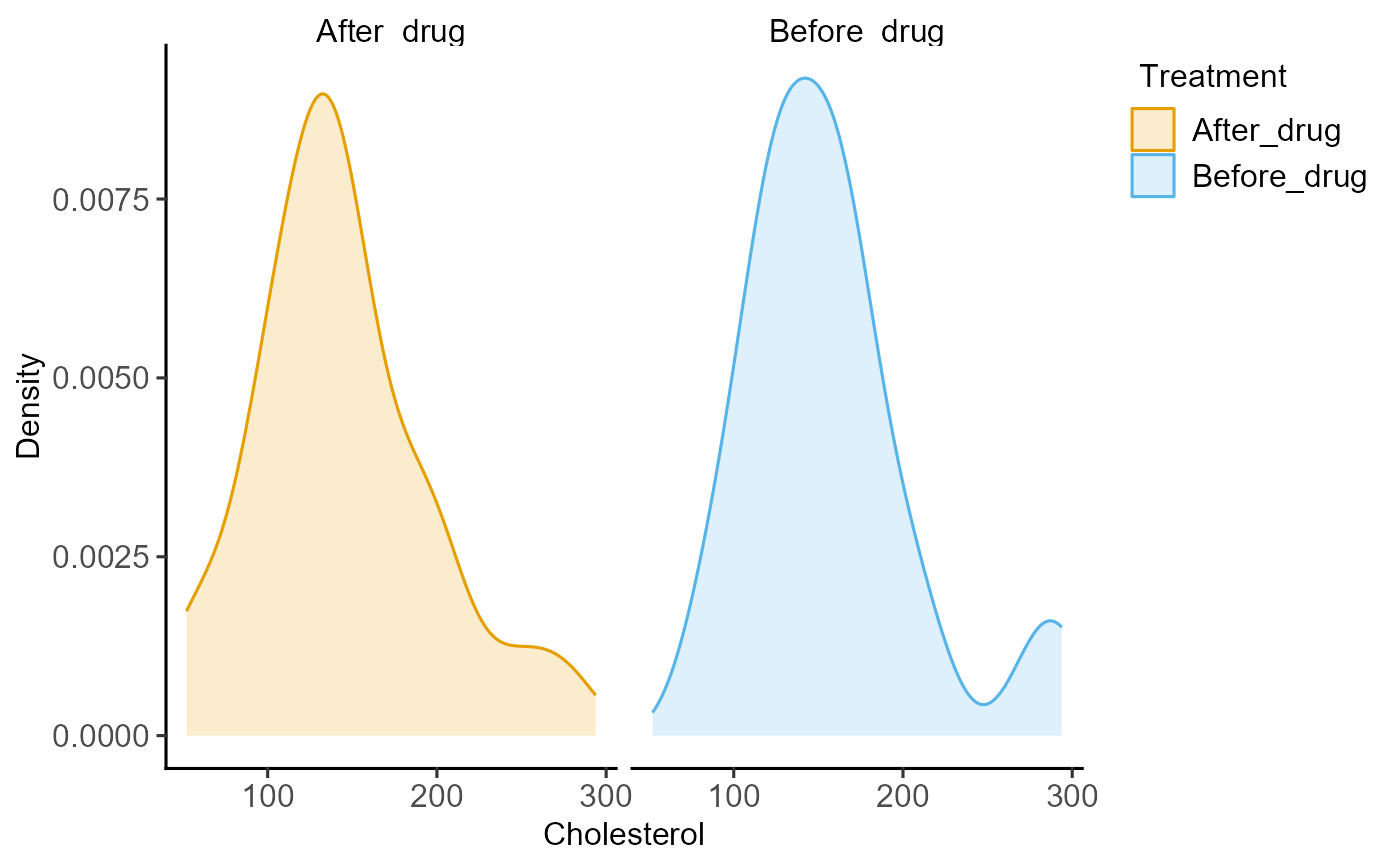
 #with faceting
plot_density(data = data_cholesterol,
ycol = Cholesterol, group = Treatment,
facet = Treatment, fontsize = 12)
#with faceting
plot_density(data = data_cholesterol,
ycol = Cholesterol, group = Treatment,
facet = Treatment, fontsize = 12)
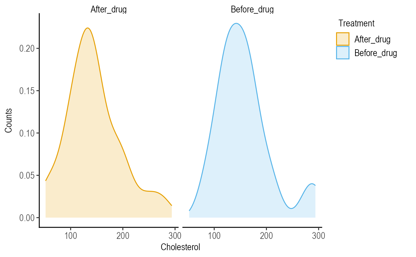
 #Counts
plot_density(data = data_cholesterol,
ycol = Cholesterol, group = Treatment,
PlotType = "Counts",
facet = Treatment, fontsize = 12)
#Counts
plot_density(data = data_cholesterol,
ycol = Cholesterol, group = Treatment,
PlotType = "Counts",
facet = Treatment, fontsize = 12)